CS180 Project2: Fun with Filters and Frequencies

1.1: Gradient Computation

To compute the image gradient, we begin by computing the partial derivatives in both the x and y directions using finite difference operators:

• The finite difference operator for the x-direction is [-1,1]
• The finite difference operator for the y-direction is [-1,1]^T

Convolving the cameraman image with these operators gives us the discrete partial derivatives ∂I/∂x and ∂I/∂y. The gradient is defined as:

∇I = √((∂I/∂y)² + (∂I/∂x)²)

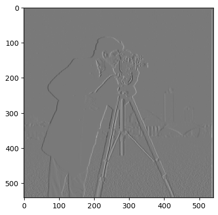
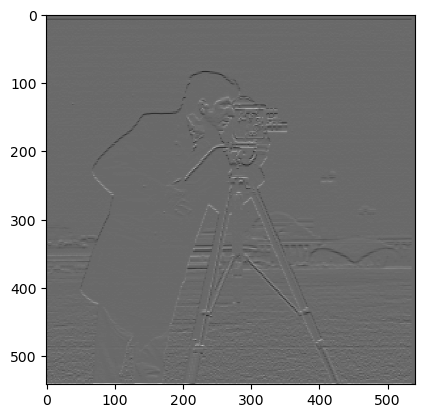
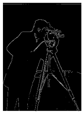
The finite difference operators are really sensitive to noise. This leads to really discrete looking edges.To reduce noise sensitivity, we use a Gaussian filter before computing the gradient. We convolve the image with a 10x10 Gaussian kernel with σ = 2.

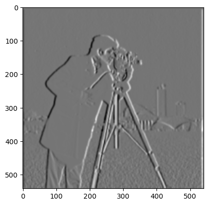
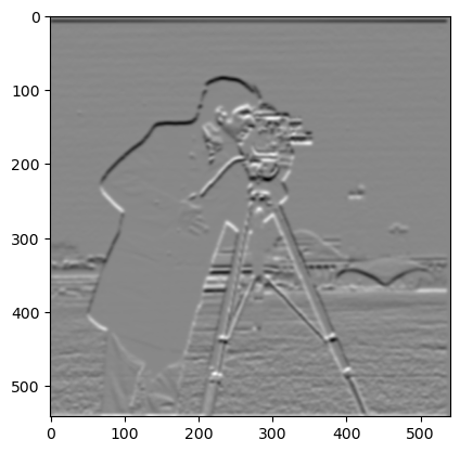
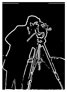
We observe that the edges detected by the gradient are much smoother in this case, compared to the non-Gaussian version.

We repeat this process again by first applying the difference operator through convolution to the gaussian followed by applying these operators to the image and then taking the sum of squares to compute the gradient. Note that by the commutative property of convolution. We expect that this image will be the same as the above, and this is exactly what we obtain. This saves us an extra convolution of the whole image which is an expensive operation.

2.1: Image Sharpening

We sharpen images by separating low and high frequencies and adding extra high frequencies back to the original image. The high frequencies are obtained by applying the Gaussian filter and subtracting this filtered image from the original image.

The sharpened image is computed as: (α + 1) * I - α * gaussian_kernel, where α controls the degree of sharpening.

Taj Mahal sharpening progression (α values 1 to 6)

Custom image sharpening progression (α values 1 to 6)

2.2: Hybrid Image

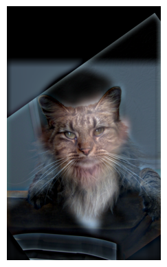
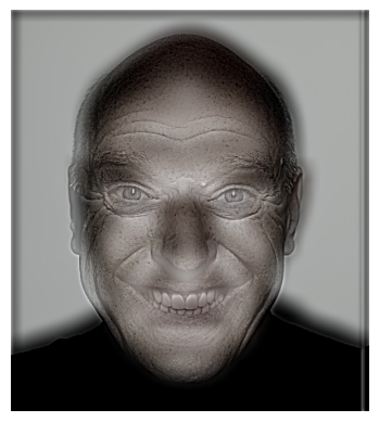
Hybrid images are created by combining low frequencies from one image with high frequencies from another. This results in an image that appears different when viewed from near and far.

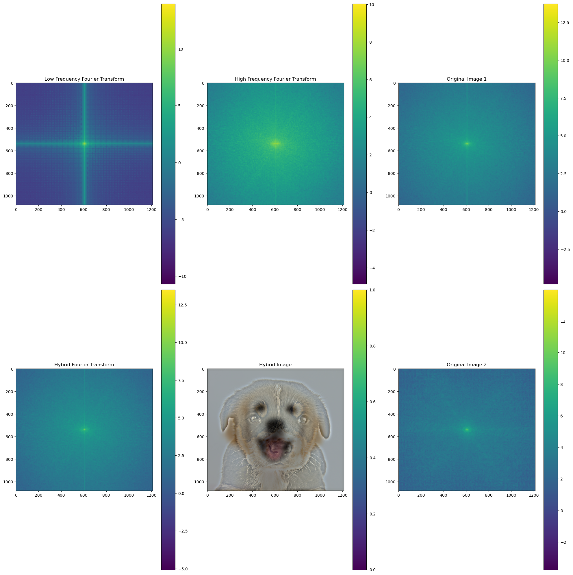
High frequencies: obtained by applying the Gaussian filter and subtracting this filtered image from the original image. Low frequencies: obtained by applying the Gaussian filter to the image.

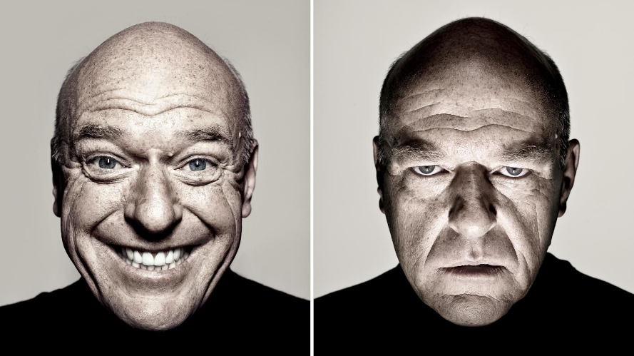
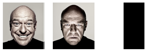
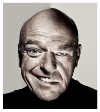
Here is the first example of a hybrid image. Note that before the images were used we used an alignment function to make sure that both the images were aligned appropriately. Here are the original pair of images and the hybrid

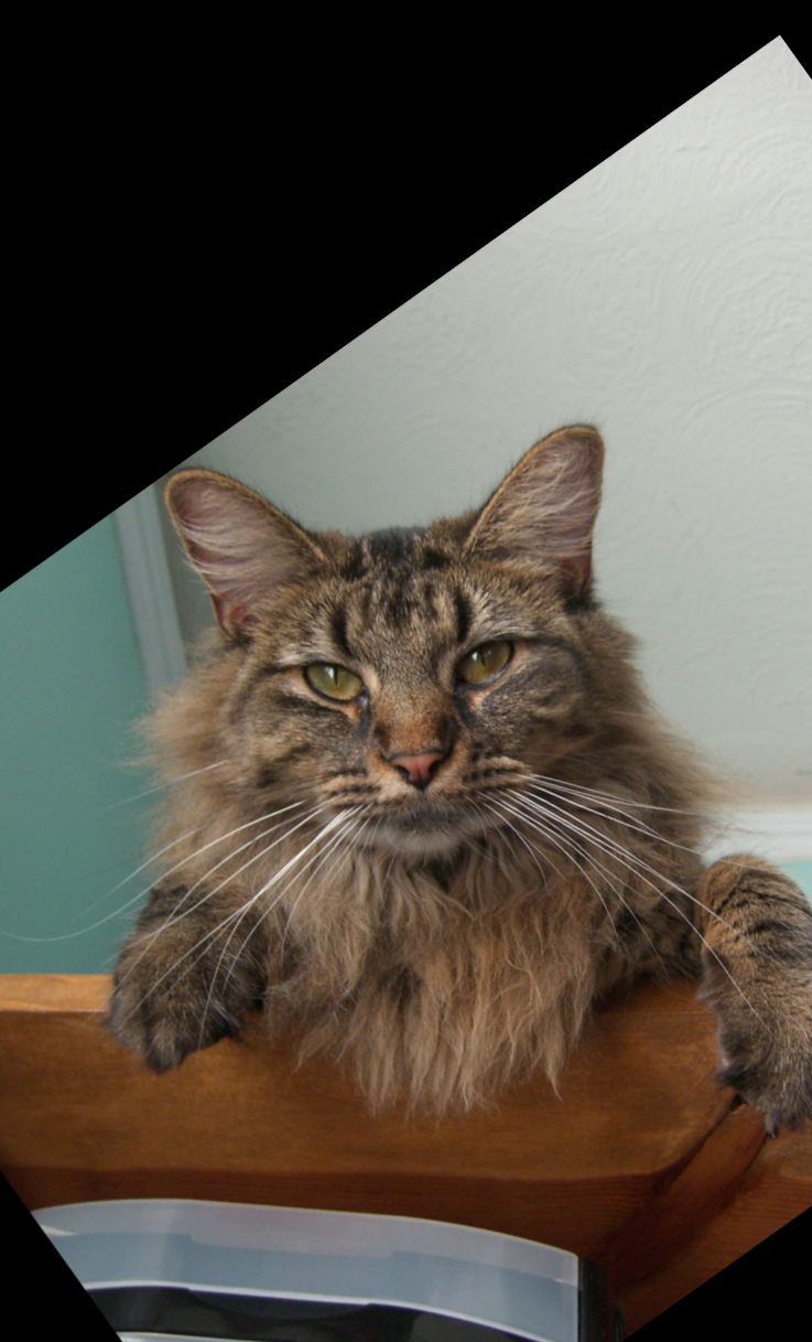
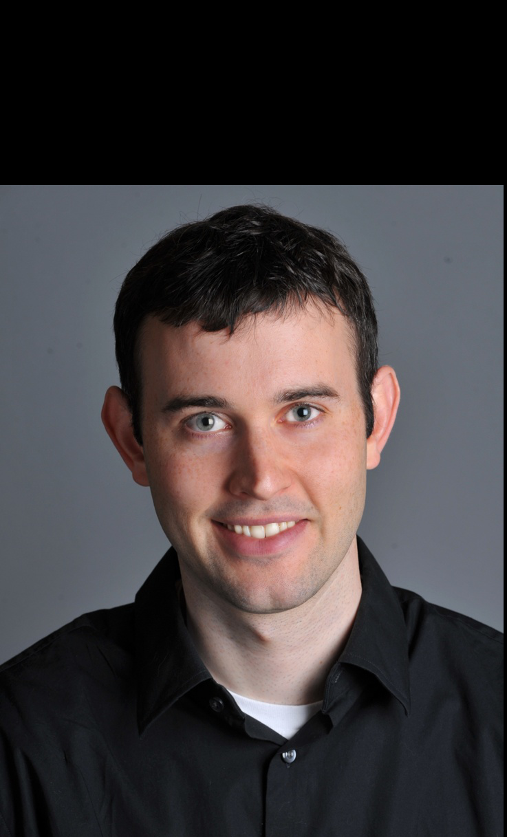
Now we have a hybrid of a happy and sad man.

Finally, we have a hybrid of a dog and a puppy.

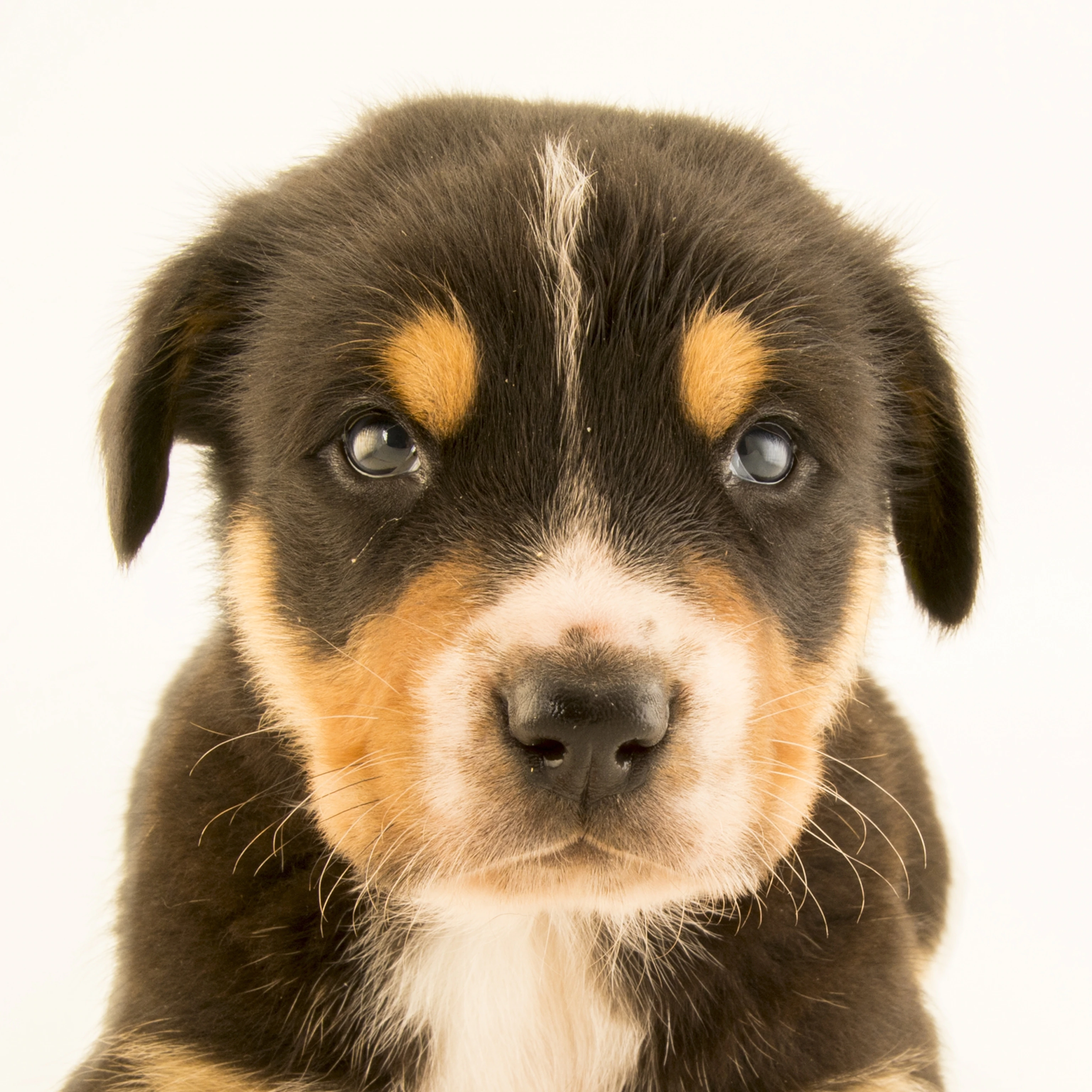
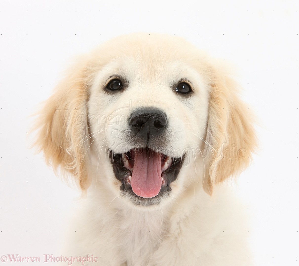
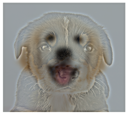
For the dog-puppy hybrid image, we also illustrate the process through frequency analysis. We convert the image using FFT into the Fourier domain to see how the low pass and high pass filters affect the result. Note that Image1 is that of the lab and Image2 is that of the puppy.

2.3: Gaussian and Laplacian Stacks

Now we move on to the problem of image blending. Note this is a stack and not a pyramid so there is no downsampling involved for pixels. The downsampling in the stack is induced by the increase of the sigma value for the gaussian kernel. The gaussian stack is created by applying the gaussian kernel with increasing values of sigma to the same image.

Laplacian stacks are generated by differencing consecutive Gaussian filtered images: Lap[i] = Gauss[i+1] - Gauss[i]. Below are the Laplacian stacks for the apple and orange images.

Here are the Gaussian stacks for the orange and apple images.:

2.4: Multiresolution Blending

We use Laplacian stacks to blend two images. The process involves:

1. Computing Laplacian stacks for both images
2. Generating a mask and computing its Gaussian stack
3. Computing merge[i] = mask[i]*im1_L[i] + (1-mask[i])*im2_L[i]
4. Summing every frame in the merge frame to obtain the final image

Here is the merged stack for the oraple:

Note the last element here is the final image of the gaussian stack. By adding this stack we get the merged image. Here is the merged image for the orange and apply

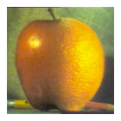
Here are some more examples of multiresolution blending:

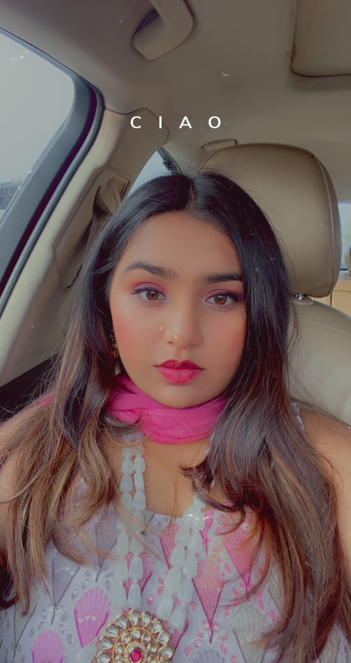
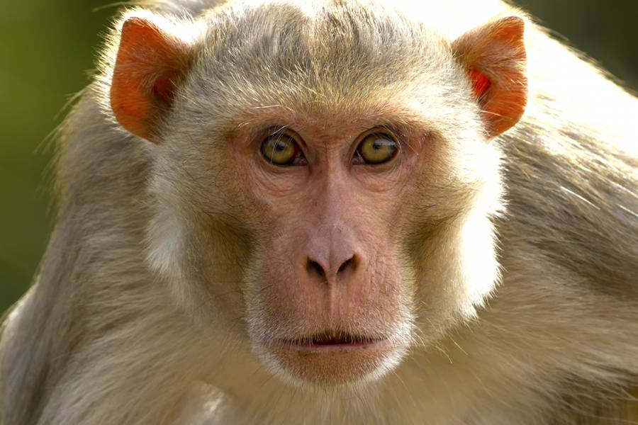
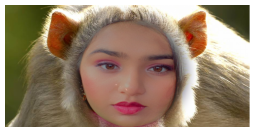
Note for this the mask was drawn by hand on a ipad