CS180 Project 5:Diffusion Models

Part 0: Sampling from the Model

The seed used for Part A was 222

In this part, you will sample images from the diffusion model. The code generates images by sampling from the model with varying numbers of inference steps. Examining three sets of images generated with 20, 40, and 100 inference steps reveals a clear increase in image quality.

20 Steps

40 Steps

100 Steps

Part 1: Sampling Loops

Part 1.1: Forward Process

The forward process is implemented using the equation:

x_t = √(ᾱ_t) x_0 + √(1 - ᾱ_t) ε, where ε ∼ N(0, 1)

This process adds Gaussian noise to an image while reducing the influence of the original image.

Timestep	Description	Image
t = 0	Original image.
t = 250	The tower remains visible, but random noise begins to affect clarity, especially in the sky and edges.
t = 500	Noise obscures much of the tower's shape, with colorful static making details hard to discern.
t = 750	The image is almost entirely noise, with only a faint outline of the tower visible.

Part 1.2: Gaussian Denoising

Applied Gaussian blur filtering to denoise image I did this for the noise values [250, 500, 750]. This clearly shows that this method is not effective at denoising

Part 1.3: One-Step Denoising

Utilized our pretrained UNet model to estimate and remove noise in just one step. We see that this does much better than the Gaussian denoising

Part 1.4: Iterative Denoising

The above one-step denoising does well but there is still room for improvement. To better this method: we will use iterative denoising to recover clean images from noisy inputs using strided timesteps. Using a stride of 30 timesteps from 990 down to 0, we can observe an improvement in image quality. The results clearly show how multiple smaller denoising steps produce significantly better results than attempting to denoise in a single large step. We will compare iterative denoising with one-step denoising and classical denoising

Noise 40

Noise 240

Noise 390

Noise 540

Noise 690

Now all three together:

Gaussian

One-Step

Iterative

Part 1.5: Diffusion Model Sampling

The model, prompted with "a high-quality photo," transforms Gaussian noise into an image by iteratively removing noise based on patterns from its training data. Each step brings the output closer to the natural image manifold.

Image 1

Image 2

Image 3

Image 4

Image 5

Part 1.6: Classifier-Free Guidance

CFG improves image generation by blending two noise estimates:

Conditional: Based on the prompt: "a high quality photo".
Unconditional: Based on an empty prompt "".

The estimates are combined using the formula:

noise_est = noise_est_uncond + cfg_scale * (noise_est_cond - noise_est_uncond)

With cfg_scale > 1, we get higher quality images aligned with the prompt.

The iterative_denoise_cfg function achieves this by:

Running the UNet model twice per step: once with prompt embeddings, once with null embeddings.
Combining predictions using the CFG formula before applying each denoising step.

For the images below, we used cfg_scale = 7.

Image 1

Image 2

Image 3

Image 4

Image 5

Part 1.7: Image Translation and Conditioning

Part 1.7.1: Editing hand drawn and web images

we take a real image, add noise to it, and then denoise. This effectively allows us to make edits to existing images. The more noise we add, the larger the edit will be. This works because in order to denoise an image, the diffusion model must to some extent "hallucinate" new things -- the model has to be "creative."

Here, we're going to take the original test image, noise it a little, and force it back onto the image manifold without any conditioning. Effectively, we're going to get an image that is similar to the test image

We test a range of starting indices [1, 3, 5, 7, 10, 20] that correspond to different levels editing.

start index 1 noise

start index 3 noise

start index 5 noise

start index 7 noise

start index 10 noise

start index 20 noise

Original

Now for two hand drawn images

start index 1 noise

start index 3 noise

start index 5 noise

start index 7 noise

start index 10 noise

start index 20 noise

Original

start index 1 noise

start index 3 noise

start index 5 noise

start index 7 noise

start index 10 noise

start index 20 noise

Original

Part 1.7.1: Inpainting

This method lets you edit an image using a binary mask. Given:

Original Image: x_orig
Binary Mask: m

The result keeps the original content where m = 0 and generates new content where m = 1.

How It Works

Run the diffusion denoising loop.
At each step, update the image to match the original where m = 0.

The update rule is:

x_t ← m * x_t + (1 - m) * forward(x_orig, t)

This ensures that the unmasked areas retain the original image while the masked areas are updated with new content.

Example

Use this method to inpaint specific parts of an image, such as restoring the top of the Campanile in a photo.

The test image

Campanile

Mask

To replace

InPainted

Capybara

Mask

To replace

InPainted

Water Bottle

Mask

To replace

InPainted

Part 1.7.3: Text-Conditioned Image-to-image Translation

In this section, we extend the previous technique by guiding the image projection using a text prompt. This allowing more specific edits beyond just projecting to the natural image manifold.

How It Works

Instead of using the default prompt "a high quality photo", we have specified custom text prompt to guide the projection.

Edited versions of the test image, using the given prompt at noise levels: [1, 3, 5, 7, 10, 20].

capybara image to dog prompt: "a photo of a dog"

capybara

390 noise

690 noise

780 noise

840 noise

900 noise

960 noise

waterbottle image to barista prompt:'a photo of a hipster barista'

waterbottle

390 noise

690 noise

780 noise

840 noise

900 noise

960 noise

Campanile image to rocket prompt: "a rocket ship"

Campanile

390 noise

690 noise

780 noise

840 noise

900 noise

960 noise

Part 1.8 Visual Anagrams

We will now generate images that look like one thing but, when flipped upside down, reveal something else. In this example, we will generate an image that looks like "an oil painting of an old man" but, when flipped upside down, reveals "an oil painting of people around a campfire."

How It Works

The process involves denoising an image in two ways, combining the results to create the illusion:

Denoise the image x_t at step t using the prompt "an oil painting of an old man", obtaining the noise estimate ε₁.
Flip the image upside down and denoise it with the prompt "an oil painting of people around a campfire", yielding the noise estimate ε₂.
Flip ε₂ back to align it with ε₁.
Average the two noise estimates: ε = (ε₁ + ε₂) / 2.
Perform a reverse diffusion step using the averaged noise estimate ε.

The algorithm can be summarized as:

    ε₁ = UNet(x_t, t, p₁)
    ε₂ = flip(UNet(flip(x_t), t, p₂))
    ε  = (ε₁ + ε₂) / 2

Here are the results:

prompt1 = "an oil painting of an old man" prompt2 = "an oil painting of people around a campfire"

Old man

People around a camp fire

prompt1 = 'a wild baboon' prompt2 = 'a volcano eruption'

Baboon

volcano erupting

prompt1 = 'a ski lift with a mountain background' prompt2 = 'a row boat in venice'

boat

ski-lift

Part 1.9: Hybrid Images

To create hybrid images using a diffusion model, we blend low frequencies from one noise estimate with high frequencies from another. Here’s the step-by-step process:

Estimate noise ε₁ for the first prompt using the UNet model.
Estimate noise ε₂ for the second prompt using the same model.
Combine the noise estimates:
- Apply a low-pass filter (e.g., Gaussian blur) to ε₁.
- Apply a high-pass filter to ε₂.
- Add the results: ε = f_lowpass(ε₁) + f_highpass(ε₂).

The algorithm can be summarized as:

    ε₁ = UNet(x_t, t, p₁)
    ε₂ = UNet(x_t, t, p₂)
    ε  = f_lowpass(ε₁) + f_highpass(ε₂)

prompt1 = "a lithograph of a skull"
prompt2 = "a lithograph of waterfalls"

prompt1 = "a rocket ship"
prompt2 = 'a pencil'

prompt1 = 'a man wearing a hat'
prompt2 = 'a volcano eruption'

Part 2: Training Diffusion Networks

In this part of the project we endeavor to structure and train our own diffusion models using pytorch on the MNIST digits dataset. We will structure this into the following steps:

Setting up the UNet Structure.
Using the UNet to Train a Denoiser
Adding Time Conditioning to UNet
Training the UNet
dding Class-Conditioning to UNet

Part 2.2: Noise Levels on MNIST digits

We will start by adding noise to the MNIST digits dataset. We will add noise at different levels to the images and visualize this.

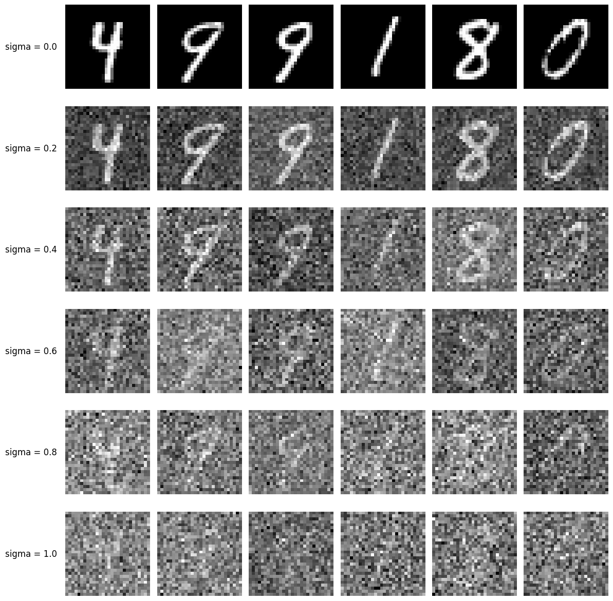
Noised MNIST digits

Part 2.2.1: Training the model to perform denoising

We will now train the model to perform denoising on the MNIST digits dataset. We will train the model to remove noise from the images. Here is the loss curve for the model:

Train a denoiser to denoise noisy image z with sigma=0.5 applied to a clean image x.

Dataset and dataloader:

Use the MNIST dataset via torchvision.datasets.MNIST with flags to access training and test sets
batch size: 256
Train for 5 epochs

hidden dimension D = 128

Adam optimizer
Learning rate: 1e-4

Here is the loss curve for the model:

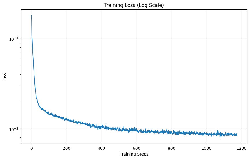
Loss curve

Here are the results on some of the MNIST images in the test set

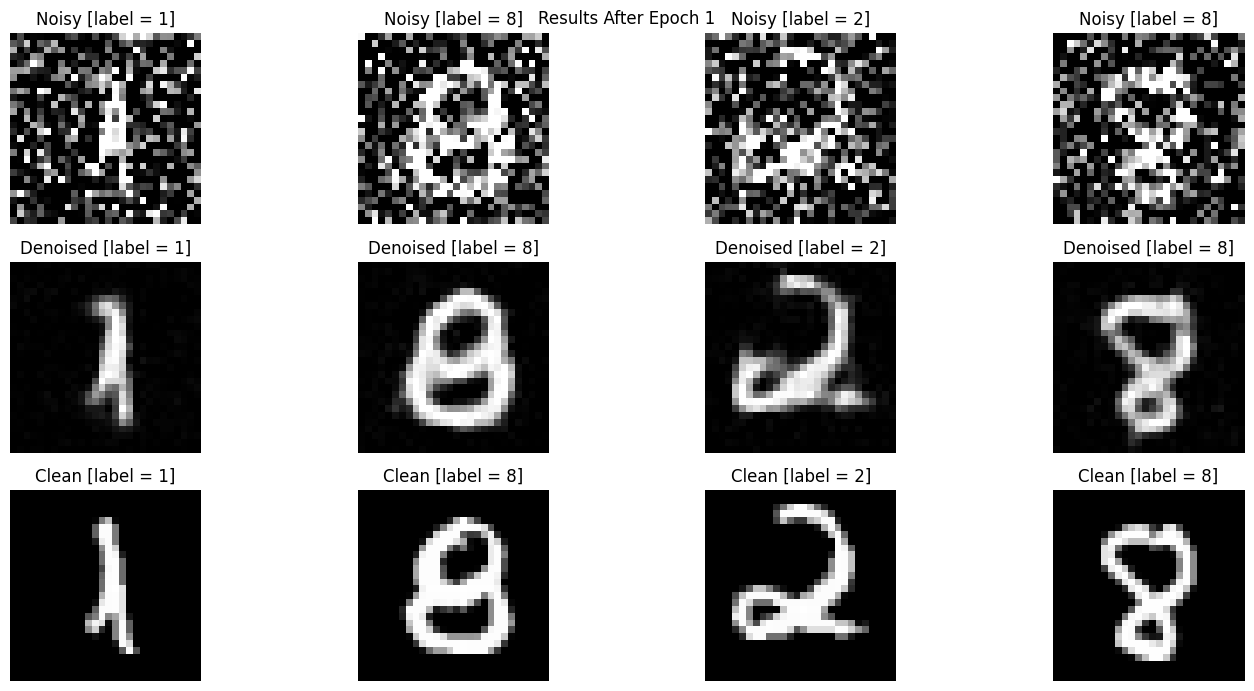
After Epoch 1

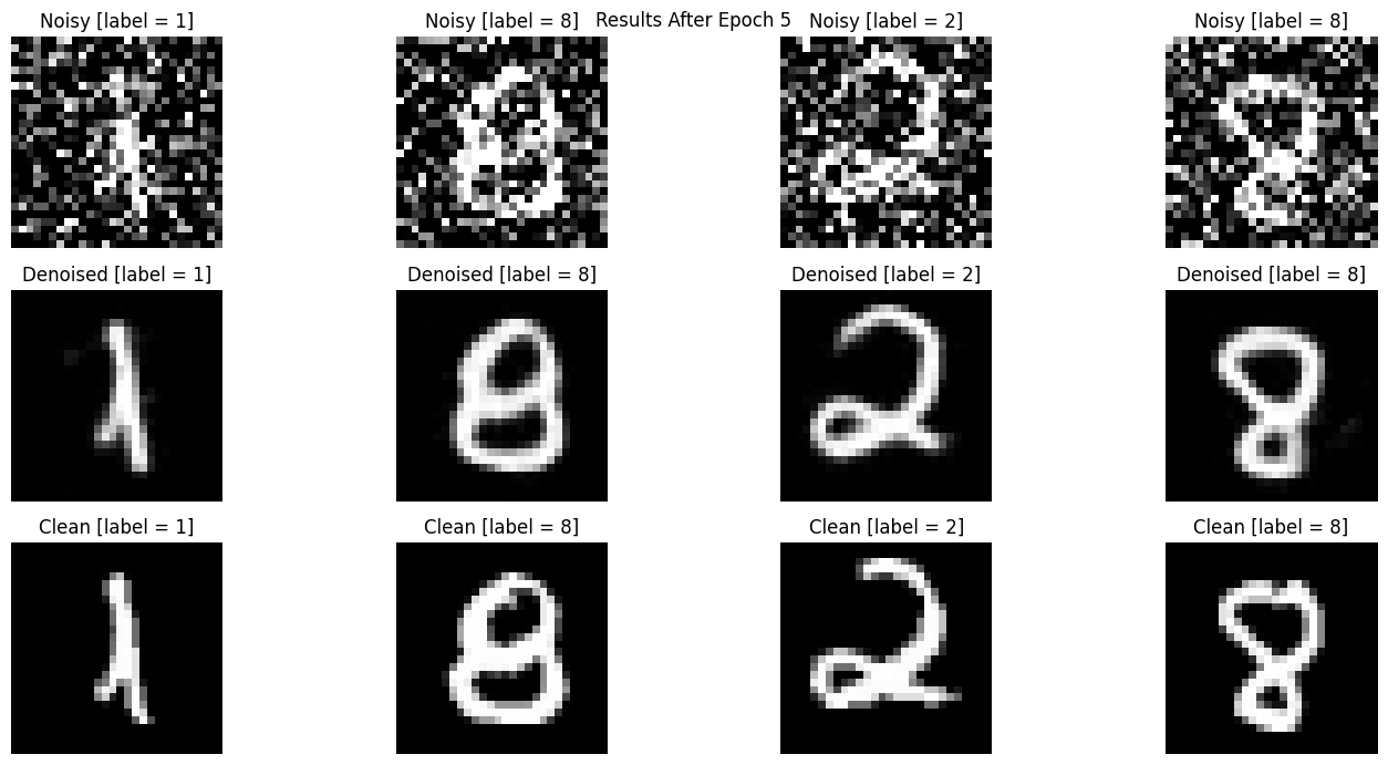
After Epoch 5

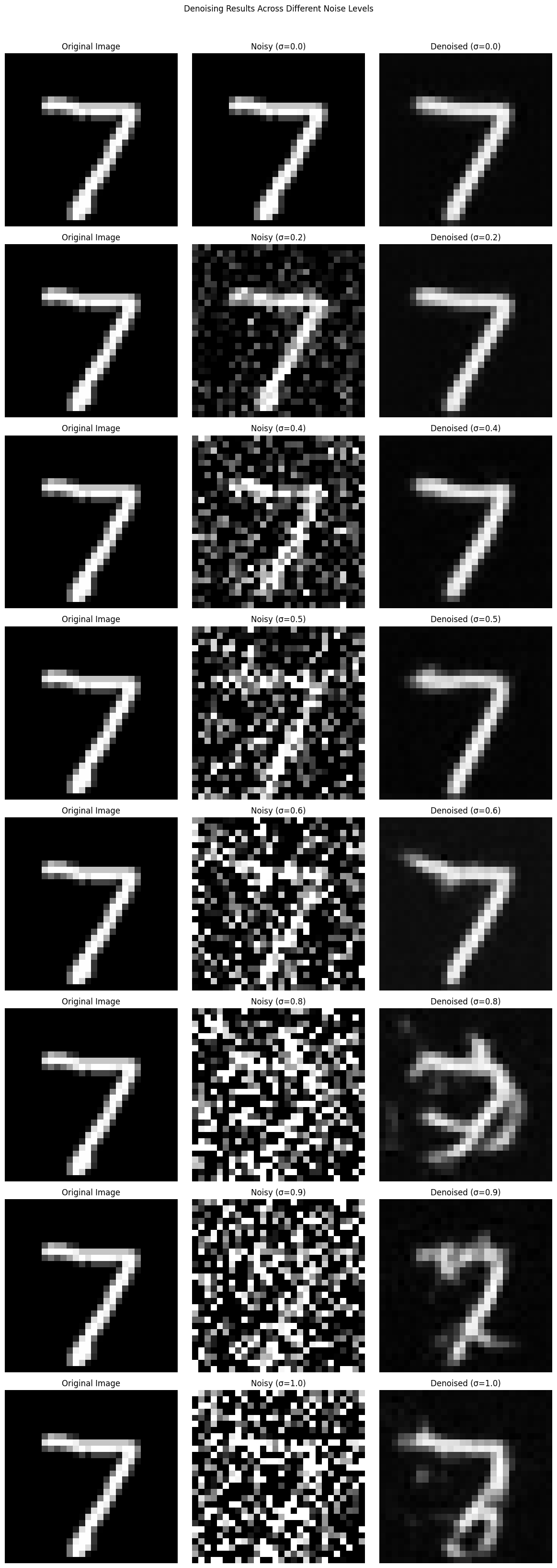
Note that our denoiser is trained on sigma = 0.5, Let's see how the denoiser performs on different sigmas that it wasn't trained for.

Part 2.2: Adding Time Conditioning to UNet

Now we move on training the diffusion models. We begin by adding time conditioning the the UNet structure and training the model.

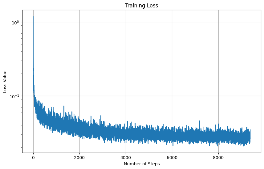
Here is the training loss curve for the UNet with time conditioning:

Here are the results on some of the MNIST images in the test set

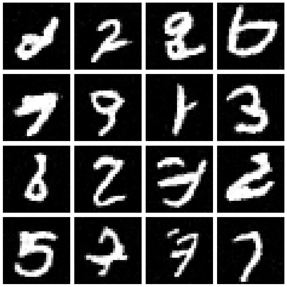
After Epoch 5

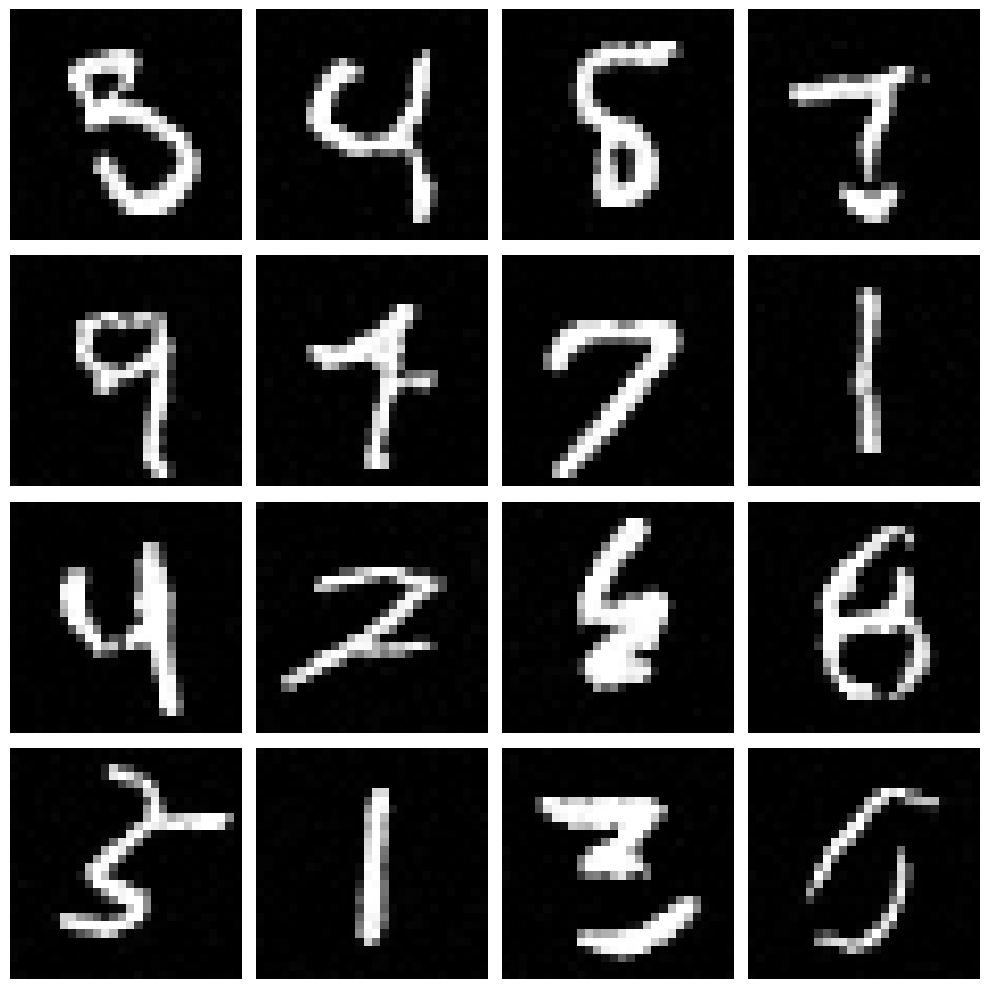
After Epoch 20

Part 2.4: Adding Class Conditioning to UNet

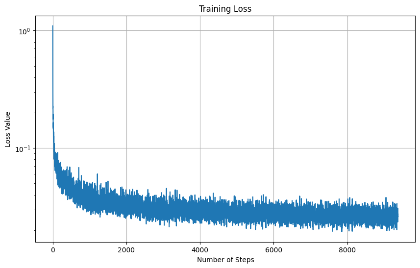
Now we move on training the diffusion models. We begin by adding class conditioning the the UNet structure and training the model. Here is the training loss curve for the UNet with class conditioning:

Here are the results on some of the MNIST images in the test set

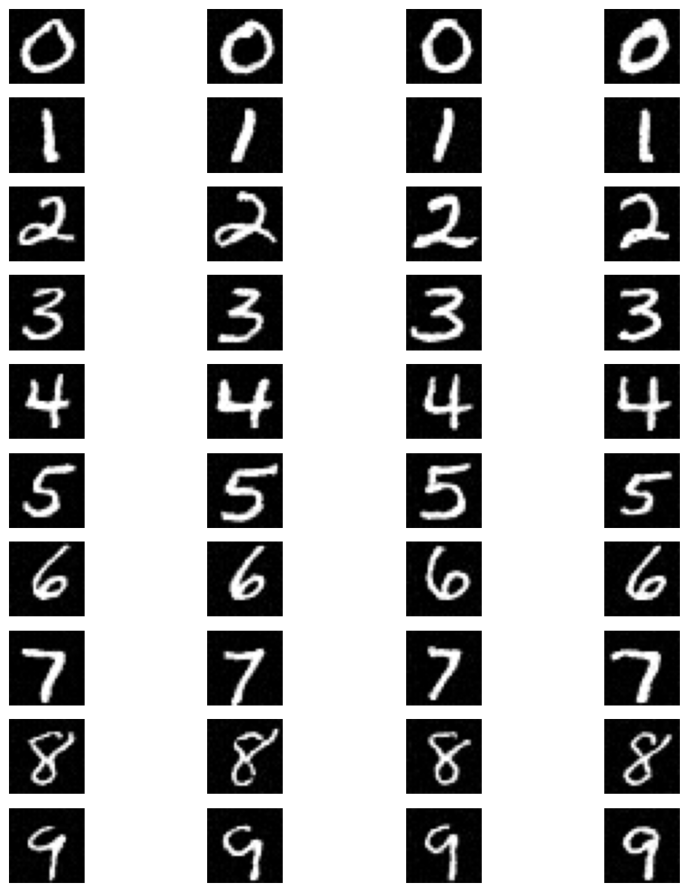
After Epoch 5

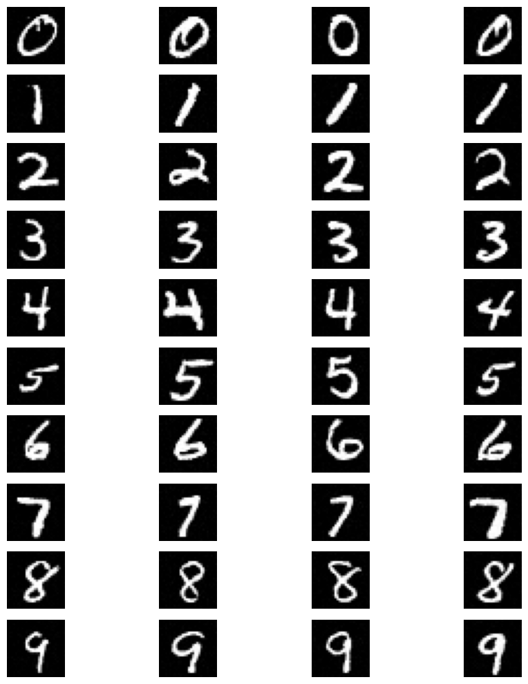
After Epoch 20